Introduction
In a previous post we discussed the backpropagation algorithm, and saw how it provides a modular and efficient way to calculate the gradient of the loss with respect to any of parameter of a deep, multi-layered neural network. We saw how a neural network can be represented as a computation graph, where each node only needs to know how to compute its own forward and backward steps. This allowed us to create neural networks of arbitrary complexity while still being able to compute the gradients required for optimizing them.
In this post, we’ll go through a practical example and see how we can define our own custom nodes in a computation graph, using PyTorch’s autograd. We’ll implement the forward and backward operations ourselves to see how all PyTorch’s built-in differentiable operations actually work behind the scenes.
We’ll also visualize the resulting computation graphs, to get a strong intuition for how the various concepts come together.
References
This post is based on materials created by me for the CS236781 Deep Learning course at the Technion between Winter 2019 and Spring 2022. To re-use, please provide attribution and link to this page.
Autograd
The torch.autograd module provides the PyTorch implementation of automatic differentiation. It allows us to define functions that can be composed into a fully differentiable computation graph.
We’ll now learn how to use PyTorch’s autograd to define our own custom functions, which can then become nodes in any computation graph.
Let’s first introduce a cousin of ReLU, the Exponential-Linear Unit (ELU) activation function:
We’ll pretend PyTorch does not include this activation function and implement a custom version ourselves.
import torch
import torch.autograd as autograd
import torchviz

from torch import Tensor
As a starting point, we’ll implement the actual computation of ELU as a standalone function so that we can reuse it later.
def elu_forward(z: Tensor, alpha: float):
    elu_positive = z
    elu_negative = alpha * (torch.exp(z) - 1)
    elu_output = torch.where(z>0, elu_positive, elu_negative)
    return elu_output
A quick visualization to see what the function looks like:
z = torch.linspace(-5, 5, steps=1000)
plt.plot(z.numpy(), torch.relu(z).numpy(), label='ReLU(z)', linewidth=5);
plt.plot(z.numpy(), elu_forward(z, alpha=.5).numpy(), label='ELU(z)', linewidth=2); plt.legend(); plt.grid();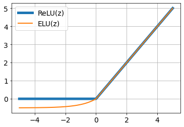
Now we’ll wrap it as an nn.Module so that we can use it as a layer in a model: we simply need to call our function in the module’s forward(). We discussed PyTorch’s modules in a previous post.
class ELU(torch.nn.Module):
    """ ELU Activation layer """

    def __init__(self, alpha: float = 0.1):
        super().__init__()
        self.alpha = alpha

    def forward(self, z: Tensor):
        return elu_forward(z, self.alpha)
Let’s use torchviz to take a look at the computation graph representing our module.
elu = ELU(alpha=0.5)
z = torch.tensor([-2., -1, 0, 1, 2, 3], requires_grad=True)
torchviz.make_dot(elu(z), params=dict(z=z))
We can see that the computation graph accurately represents the various basic mathematical operations performed by our elu_forward function (ignore the Backward0 suffixes for now).
Custom autograd functions
What if we wish to define the entire ELU operation as one node in the graph? This can be useful in various cases, such as:
- Performance optimization: a complex forward pass with a simple analytical gradient might benefit from a custom backward implementation.
- If PyTorch can’t differentiate through our layer properly. In a future post, we’ll see an example of this, in the context of differentiable optimization.
- If we need to produce a “wrong” gradient for some reason. This is used e.g. for adversarial losses that use gradient reversal (another topic for a future post).
How might we accomplish this? We’ve observed that by simply using the built-in PyTorch operations to implement the ELU’s forward pass, we already create a differentiable graph composed of each individual operation.
To create a single node that represents the entire ELU, we need a way to tell PyTorch not just about its forward operation, but also about the backward pass, which means calculating the derivative of ELU.
We must use a lower-level PyTorch API, autograd.Function,
which allows us to define an operation in terms of both its forward pass
(the regular output computation), and also its backward pass
(the gradient w.r.t. all of its inputs).
From the PyTorch docs:
Every operation performed on
Tensorss creates a newFunctionobject, that performs the computation, and records that it happened. The history is retained in the form of a DAG of functions, with edges denoting data dependencies (input < output). Then, when backward is called, the graph is processed in the topological ordering, by callingbackward()methods of eachFunctionobject, and passing returned gradients on to nextFunctions.
The API of an autograd.Function is:
class MyCustomFunction(autograd.Function):

    @staticmethod
    def forward(context, *inputs: Tensor, **kw):
        ...

    @staticmethod
    def backward(context, *grad_outputs: Tensor) -> Sequence[Tensor]:
        ...
The autograd.Function API contains a few interesting details, which are crucial to notice if we would like to truly understand how backpropagation works. Let’s consider three details in particular. Try to answer the following questions based on your understanding of backpropagation.
What does grad_outputs contain?
This is the input to the backward pass, which means it must be the gradients (of the downstream loss) with respect to the outputs of the current function (e.g. ELU). This is what’s required to apply the chain rule at the current node.
Consider that our function is
What does the backward() method return?
Since this is the output of the backward pass, it should return the gradient of the loss with respect to each of the tensors in *inputs, which are the inputs to our function. In our previous example, the *inputs would contain backward() function needs to return
Why do we need the context argument?
This is a subtle detail that is mainly related to the implementation, and may not be immediately obvious from the math. The short answer is that context contains any saved data from the forward pass that is required to compute
Notice that both the forward() and backward() methods are marked with the @staticmethod decorator, meaning they cannot access any class state. Therefore, all the information required to compute these function’s results (function parameters, input arguments, and gradients of outputs) must be provided directly at call time via the *inputs and *grad_outputs arguments.
To see when this might be needed, let’s consider a simple example. Suppose our function is just a linear layer with a single output:
This means that in the backward() function, we must know the values of context object allows us to save it during the forward pass, and it will be automatically available for us during the backward pass. In the next section, we’ll see an example of how this works.
ELU as a custom function
To implement the ELU as an autograd.Function, we’ll first calculate the derivative of the ELU function analytically:
Next, we need to figure out how to compute the vector-Jacobian product (VJP) efficiently, given
Since the Jacobian is a diagonal matrix, it follows that the VJP can be computed as a simple elementwise multiplication of vectors:
Now, equipped with the expression for the VJP, we have all that’s required to implement the Function object representing ELU. Try to follow the implementation below. The comments explain exactly what’s happening in each line, and how it relates to the discussion above. Notice also how the context (ctx in the code) is used to pass parameters from the forward to the backward.
class ELUFunction(autograd.Function):

    @staticmethod
    def forward(ctx, z: Tensor, alpha: float):
        elu = elu_forward(z, alpha) # Regular forward pass computation from before
        ctx.save_for_backward(z)    # Tensors should be saved using this method
        ctx.alpha = alpha           # other properties can be saved like so
        return elu

    @staticmethod
    def backward(ctx, grad_output):
        z, = ctx.saved_tensors      # Validates that no in-place modifications happened on saved tensors
        alpha = ctx.alpha

        # Calculate diagonal of d(elu(z))/dz
        grad_positive = torch.ones_like(z)
        grad_negative = alpha * torch.exp(z)

        # Note: This is not the full Jacobian, d(elu(z))/dz, it's the diagonal
        grad_elu = torch.where(z>0, grad_positive, grad_negative)

        # Gradient of the loss w.r.t. our output
        δ_elu = grad_output

        # Calculate δz = d(elu(z))/dz * δ_elu
        # Note: elementwise multiplication equivalent to vector-Jacobian product
        # Also return None for the second input (alpha) which doesn't require gradients.
        δz = grad_elu * δ_elu
        return δz, None
Using custom functions
We can now use this custom Function either directly or as part of a layer. Note that we don’t call the forward(), method directly, but instead use Function.apply(). This tells PyTorch to create a new context, and call our function’s forward(), and insert its backward() into the computation graph, accepting the same context object.
Here’s an ELU layer (nn.Module) that uses our custom backward (via autograd.Function):
class ELUCustom(torch.nn.Module):
    """ ELU Layer with a custom backward pass """

    def __init__(self, alpha: float = 0.1):
        super().__init__()
        self.alpha = alpha

    def forward(self, z: Tensor):
        # Function.apply() invokes the forward pass with a new context
        # and updates the computation graph of the inputs
        return ELUFunction.apply(z, self.alpha)
elu_custom = ELUCustom(alpha=0.5)
z = torch.tensor([-2., -1, 0, 1, 2, 3], requires_grad=True)
torchviz.make_dot(elu_custom(z), params=dict(z=z))
Notice how the computation graph no longer contains the backward step of all the intermediate mathematical operations that were required to compute ELU. Instead, it has just a single backward function, ELUFunctionBackward which represents our custom backward pass implementation.
The code snippet above only tested the forward pass. Let’s now put our custom layer in the context of a larger model and see that we can backprop through it. We’ll define a simple MLP with ELU activations between the layers.
elu_mlp = torch.nn.Sequential(
    torch.nn.Linear(in_features=512, out_features=1024),
    ELUCustom(alpha=0.01),
    torch.nn.Linear(in_features=1024, out_features=1024),
    ELUCustom(alpha=0.01),
    torch.nn.Linear(in_features=1024, out_features=10),
    torch.nn.Softmax(dim=1)
)

elu_mlp
Sequential(
(0): Linear(in_features=512, out_features=1024, bias=True)
(1): ELUCustom()
(2): Linear(in_features=1024, out_features=1024, bias=True)
(3): ELUCustom()
(4): Linear(in_features=1024, out_features=10, bias=True)
(5): Softmax(dim=1)
)
Now we can visualize the computation graph of the full MLP.
x = torch.randn(10, 512, requires_grad=True)
torchviz.make_dot(elu_mlp(x).mean(), params=dict(list(elu_mlp.named_parameters()) + [('x', x)]))
We can notice a few interesting things in this graph:
- The weights and biases of each linear layer are visible in blue.
- There’s a single
AddmmBackwardper linear layer, representing the backward pass of2 in a single graph block, instead of separate blocks for the multiplication and addition. This is probably done for performance reasons. - The tensors we saved in the
contextof our custom function are shown in orange.
Finally, let’s run a backward pass and make sure we have gradients on all parameter tensors of our MLP.
l = torch.sum(elu_mlp(torch.randn(10, 512, requires_grad=True)))
l.backward()

for name, param in elu_mlp.named_parameters():
    print(f"{name} {torch.norm(param.grad).item()}")
0.weight 2.1810672024002997e-07
0.bias 8.488709291043506e-09
2.weight 2.8359423254187277e-07
2.bias 1.8296777426485278e-08
4.weight 2.634928648603818e-07
4.bias 3.7974928090989124e-08
Seeing gradients computed for all the network parameters shows us that PyTorch’s autograd has successfully backpropagated through our custom ELU implementation.
Conclusions
In this post, we went through a concrete technical example of implementing both the forward and backward operations required for the construction of a differentiable computation graph. This example was designed to show you exactly how backpropagation and automatic differentiation work in practice. Hopefully, the next time you see a loss.backward() call in the wild, what’s going on behind the scenes of that call will be much less mysterious :).