Optimization basics for deep learning

Introduction

Optimization is at the core of many algorithms that learn from data. It provides the basic mathematical framework for solving problems in virtually any domain. When I first heard about optimization algorithms, it sounded like a relatively dusty and obscure niche of applied math. These days, optimization has become a hot topic due to the popularity of deep learning. In deep learning, we use one particular optimization algorithm, gradient descent, to gradually update our model’s parameters until we deem our model to have “learned”.

In this post, I aim to cover the basics that are required for understanding and training deep neural networks. It’s not meant to be a mathematically rigorous review, or completely extensive. Instead, I’ll focus on the topics I find most useful in practice, without going too deeply into them. I’ll also try to provide intuitions that can help understand these topics better.

We will cover:

• Gradient descent: The core algorithm used to update model parameters.
• Various techniques to make gradient descent work in practice.
• Back-propagation: the algorithm used to calculate the gradients needed for gradient descent.

References

This post is based on materials created by me for the CS236781 Deep Learning course at the Technion between Winter 2019 and Spring 2022. To re-use, please provide attribution and link to this page.

Some images used here were taken and/or adapted from the following sources:

• Dr. Roger Grosse, UToronto, cs321
• Fundamentals of Deep Learning, Nikhil Buduma, Oreilly 2017

Descent-based optimization

Training deep neural network is performed iteratively, using descent-based optimization (see e.g. this previous post for a simple example). In this approach, we gradually update the model parameter values, each time in a way which should slightly reduce the loss. We aim to keep updating the parameters, until we find the “best” parametrization, or at least until we can’t improve the loss further.

The general scheme is,

1. Initialize parameters to some , and set .
2. While not converged:
   1. Choose a direction
   2. Choose a step size
   3. Update:

Note that by “converged” we usually mean that the loss value stops decreasing meaningfully from step to step (i.e., it changes by less than some ). True convergence would mean that we’re -close to the global optimum.

Which descent direction should we choose?

Since we aim to decrease the loss function , we could choose the direction which maximally decreases it:

Note that we limit ourselves to unit vectors, since we’re only concerned about the direction. For a fixed step size (of one unit), what is the optimal direction?

Using a first order Taylor expansion, we can write the loss at a perturbed point as,

Substituting this approximation into the optimization problem above, we find that

Which direction would minimize that expression? Since it’s an inner product between two vectors, its maximum/minimum will occur when they are co-linear. If is in the same direction as the gradient of the loss at it would maximize the inner product. Similarly, if is in the opposite direction of the gradient, it would minimize it, which is just what we need.

Using as the direction for the parameter update step results in an optimization algorithm known as gradient descent (GD).

Side note: other optimal descent directions?

The choice of -norm also matters for determining which direction is optimal. Usually, the standard Euclidean L2 norm is used (), which indeed results in being optimal.

However, other norms would produce different directions. For example, for , the L1 norm would result in being equal to the negative of the largest component of the gradient. Using this direction is known as coordinate descent.

Stochastic Gradient Descent

While gradient descent provides the theoretical foundation, computing gradients over entire datasets is computationally prohibitive. We’ll now discuss a variant of gradient descent which is used in practice.

When we write the loss as , it is to emphasize that it’s the parameters we’re optimizing for. However, obviously the loss is also a function of the data samples used to compute it.

Ideally, we’d like to minimize is the expected loss over the distribution of the data, which we can write as , where is the data sample distribution. In practice, however, we can only estimate this from the finite data at hand. If we now imagine the loss “surface” as the function , it’s clear that we will actually get different loss surfaces when we change the input data .

In stochastic gradient descent (SGD), only a single sample is considered at each optimization step . The loss on this sample is calculated, and the gradient of this single-sample loss is used as the descent direction at step : .

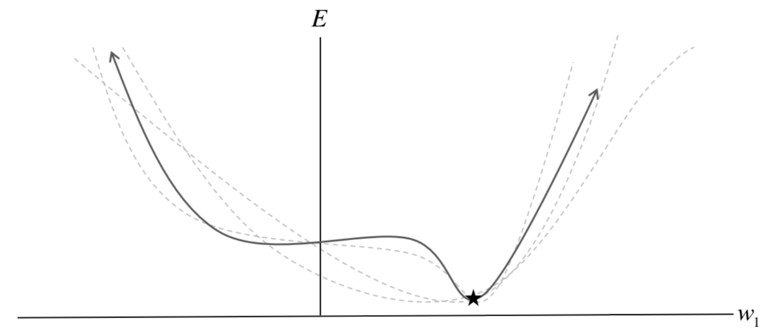
With SGD, we effectively get a different loss surface for every optimization step because a different sample is used. This can aid in convergence to a better solution because it can prevent getting stuck in bad local minima: the local minima might be there for the current sample, but not for the next one.

SGD can therefore help in mitigating the susceptibility to initialization issue with non-convex objectives. The figure illustrates this idea.

Does SGD actually converge, though? Will we get to the optimum even in the simple case of a convex loss?

It can be shown that under some conditions, SGD converges to the same (local) optimum as GD, but at a slower rate, i.e. more optimization steps are required for convergence to within the same distance from the optimum. The most important condition is we need unbiased gradients: the expected value of the stochastic gradients should be the true gradient. This holds if the parameters are independent of the data distribution.

Intuitively, we can think of the SGD gradients as “noisy”, in the sense that they don’t point exactly in the same direction as the true gradient (which is intractable to obtain). However, if there’s no bias in the sampling procedure, then the noise in the gradient directions is also unbiased and will “cancel out”, given enough samples.

The problem with SGD is that in practice, using just a single sample at a time is too noisy: convergence can be slow since these single-element gradients can sometimes point in an entirely wrong direction, making optimization erratic.

Therefore, a more commonly used variant is mini-batch SGD, where we sample a batch of samples for computing the gradient, instead of just one. Mini-batch SGD is a practical compromise: it produces less noisy gradients, which are simply the empirical average of the gradients of the multiple individual batch elements. This usually results in faster convergence, without sacrificing the benefits of SGD.

Now that we understand the basics of gradient descent, we’ll next focus on some of its drawbacks and common mitigations that are used in practice.

Susceptibility to initialization

By following the gradient, we will eventually reach a critical point, where the gradient is zero. But for general non-convex losses, there’s no guarantee that the point we reached is globally optimal. For this reason, initializing near local minima can prevent finding better ones.

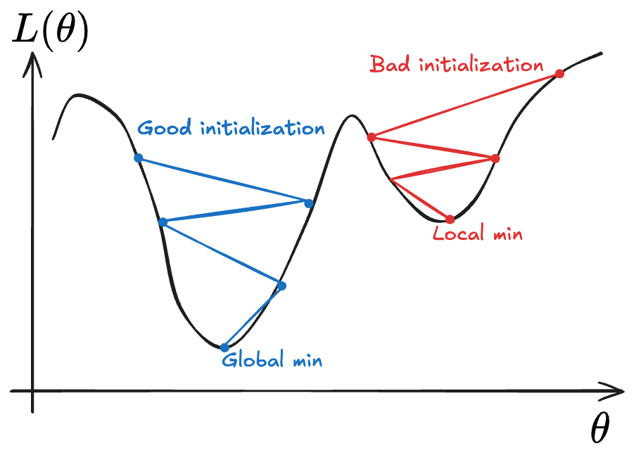There exist some “fancy” initialization techniques for the parameters of neural networks, which aim to reduce the chance of a bad initialization. We wont go into these here, but note that nothing can guarantee protection from a truly bad initialization.

One possible mitigation is LR scheduling (discussed below), which can help get out of local minima in some cases.

Sensitivity to curvature

The rate of convergence how many steps it takes to reach the optimum (or within an -ball of it) is affected by the curvature of the loss function. Intuitively, low curvature functions look more like “bowls” which have similar slopes in each direction around their minima, while high curvature means narrow “ravines” and potentially very different steepness in different directions around a minima.

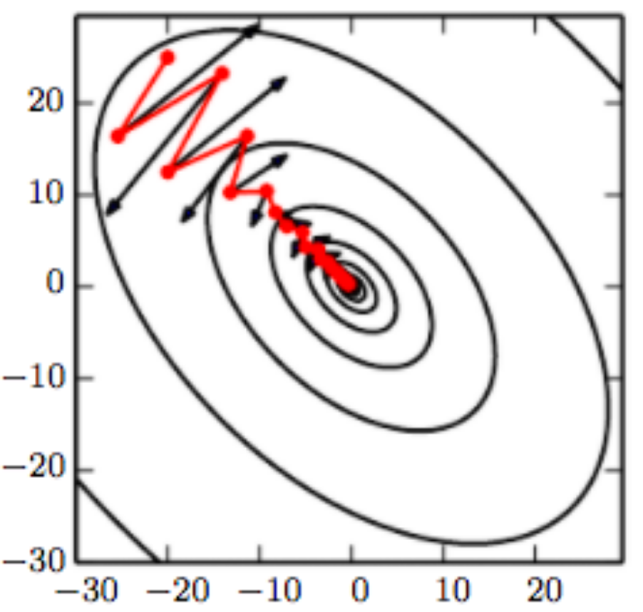
The curvature at each point can be formally defined and measured using the second derivative, or the Hessian matrix for a high-dimensional function. The curvature can be measured via the condition number where the -s are the largest and smallest eigenvalue of the Hessian matrix, . The larger , the more skewed the loss function is, and the slower convergence will become (at least around the point where was computed). The condition number determines how elongated the contours are.

Some approaches to mitigate the issue of curvature are detailed below.

Momentum

The core idea is to use a moving average of previous gradients in addition to the current gradient. This builds “speed” in the common direction, and cancel-out oscillations in opposite directions. The result is a smoother optimization trajectory and usually faster convergence.

The approach is to maintain a momentum vector that combines historical gradient information:

where is a coefficient which creates an exponential moving average of past gradients. We can think of as the “mass” or weight of a ball rolling down a hill, while the gradient is its velocity. The value of is typically chosen around 0.9, giving much more weight to the past gradients, and creating an “effective memory” of steps. Since the initial momentum is , so we can see that the first step is equivalent to a standard gradient step, but subsequently previoius gradients are also included in the moving average.

A common variant of the Momentum approach is Nesterov Accelerated Gradient (NAG). The idea is to use the gradient at the next parameter values (as predicted by momentum), instead of the gradient at the current ones:

The interpretation is that we first do a step along the direction of momentum, and do a gradient step from the point we reach. This approach prevents overshooting the minimum and further reduces oscillations in the gradient.

Batch normalization

Batch Normalization is an operation typically applied right before the activation function in each layer of a deep neural network (I covered the basics of deep neural networks in a previous post).

The normalization is simple: The mean and standard deviation of each feature are calculated over the batch dimension (the model sees a batch of samples during each forward pass). The value of each feature is then updated by subtracting the mean and scaling by the standard deviation:

Where here is a batch containing a single feature, and and are its empirical mean and variance. Following this, learnable scale and shift parameters are applied:

Batch normalization reduces the amount of change in the loss function due to a perturbation of the weights. Consequently, the effective curvature of the loss surface is reduced. In practice, this technique allows for faster convergence with larger learning rates.

Second-order methods

Second-order methods directly account for curvature by using the Hessian matrix . The canonical approach is Newton’s method:

Notice that the inverse of the hessian is applied to the gradient vector before using it for the optimization step. This is called pre-conditioning, and doing it with the Hessian makes a skewed loss surface around become bowl-shaped, i.e. it has the same curvature in all directions.

This only works when the Hessian is positive definite, which means that we are in the region of a local minimum. Otherwise, this approach can lead us in the wrong direction. In practice, a regularization term is usually added, to ensure positive definiteness: .

Second order methods, based on Hessian estimation, are typically not used with large neural networks (millions of parameters) because computing the full Hessian requires time per forward/backward pass, and inverting it requires .

Sensitivity to learning rate

Another important issue with descent-based optimization is that we need to choose the step size , also known as the learning rate. A learning rate that’s too small would hinder our convergence rate (requiring many more optimization steps); too large and we might never converge at all, due to “missing” the local minimas.

Theoretically, the largest “allowed” step size is related to a quantity known as the Lipschitz constant of the loss function. The Lipschitz constant is essentially an upper bound on how much the function can change in value given a small step in some direction (input perturbation). The larger the Lipschitz constant, the “steeper” teh loss function in some places, and therefore the smaller the learning rate needs to be in.

The following image illustrates this for a simple convex function.

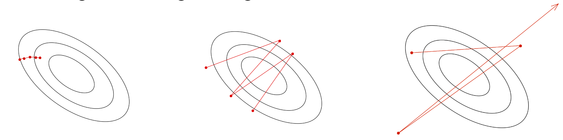
A constant step size is therefore too limiting, and in practice some strategy for updating it from step to step should be employed.

Line search

Line search is essentially 1D minimization for the optimal learning rate. Given a step direction (e.g. the negative gradient), the optimal step size in this direction, in terms of reducing the loss, is

Since this is a 1d optimization problem, there are effective methods for solving this problem. Some iterative approach is generally used in order to exponentially half the search space each iteration. There also exist approximations that ensure the overall loss is reduced, even without having to solve this problem exactly.

Learning rate scheduling

As we saw, due to the varying curvature in different parts of the loss space, it’s challenging to choose a single learning rate that works well everywhere. LR scheduling means updating the learning rate each step according to a pre-defined algorithm (the “schedule”).

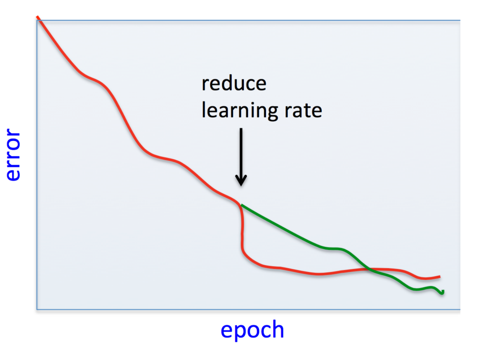
One motivation for it is that larger steps are useful at the beginning, for making rapid progress, or because we’re still far from the optimum. However, as we approach a local minimum, it might be useful to start making smaller steps so that we can get into the minima’s “ravine” instead of skipping over it. One type of LR schedule is therefor simply to decrease the learning rate each step, so that the SGD makes smaller and smaller steps as we approach the optimum.

Another motivation relates to exploration of the non-convex loss surface. We’ve discussed how SGD can get stuck in local minima and provides no guarantee about converging to a global one. If we become stuck at a local minimum, one way to get out of it is to suddenly increase the learning rate, which could make us “jump out” and resume exploring the loss surface. Therefore, another common LR scheduling approach is cyclical: decrease it for some number of steps, then increase to a new starting value (maybe lower than the original), decrease again, and repeat, in the hopes of escaping local minima.

Examples of common scheduling approaches are,

• Step decay: Reduce by a factor (e.g., 0.1) at fixed intervals.
• Exponential decay: .
• Cosine annealing: , which cycles the learning rate down from to every steps.
• Warm restarts: Decrease each step with some approach, but periodically reset to a high learning rate to escape bad local minima.

Adaptive learning rate methods

Rather than using a single global learning rate, adaptive methods maintain per-parameter learning rates that adjust based on gradient history.

Adaptive methods can be considered as a way to implement per-parameter preconditioning, which is much less computationally expensive than e.g. second order methods, while still improving optimization for regions with varying curvature more efficiently, compared to vanilla SGD.

RMSProp maintains a moving average of squared gradients, , and uses it to normalize the step size:

where is a common choice, and note that all operations are elementwise. Parameters with large typical gradients get smaller effective learning rates, while those with small gradients get larger ones. The constant is added simply for numerical stability.

Adam (Adaptive Moment Estimation) simply combines both momentum with the squared gradient moving average approach for obtaining per-parameter adaptive learning rates:

Typical values are , , . Adam has become a popular choice as a starting point, due to its reasonable convergence even with minimal hyperparameters tweaking.

The back-propagation algorithm

All the above optimization methods have a crucial thing in common: They require calculation of gradients of the loss w.r.t. to the parameters.

In practical settings when training neural networks, we have many different parameter tensors we would like to update separately. Thus, we require the gradient of the loss with respect to each of them.

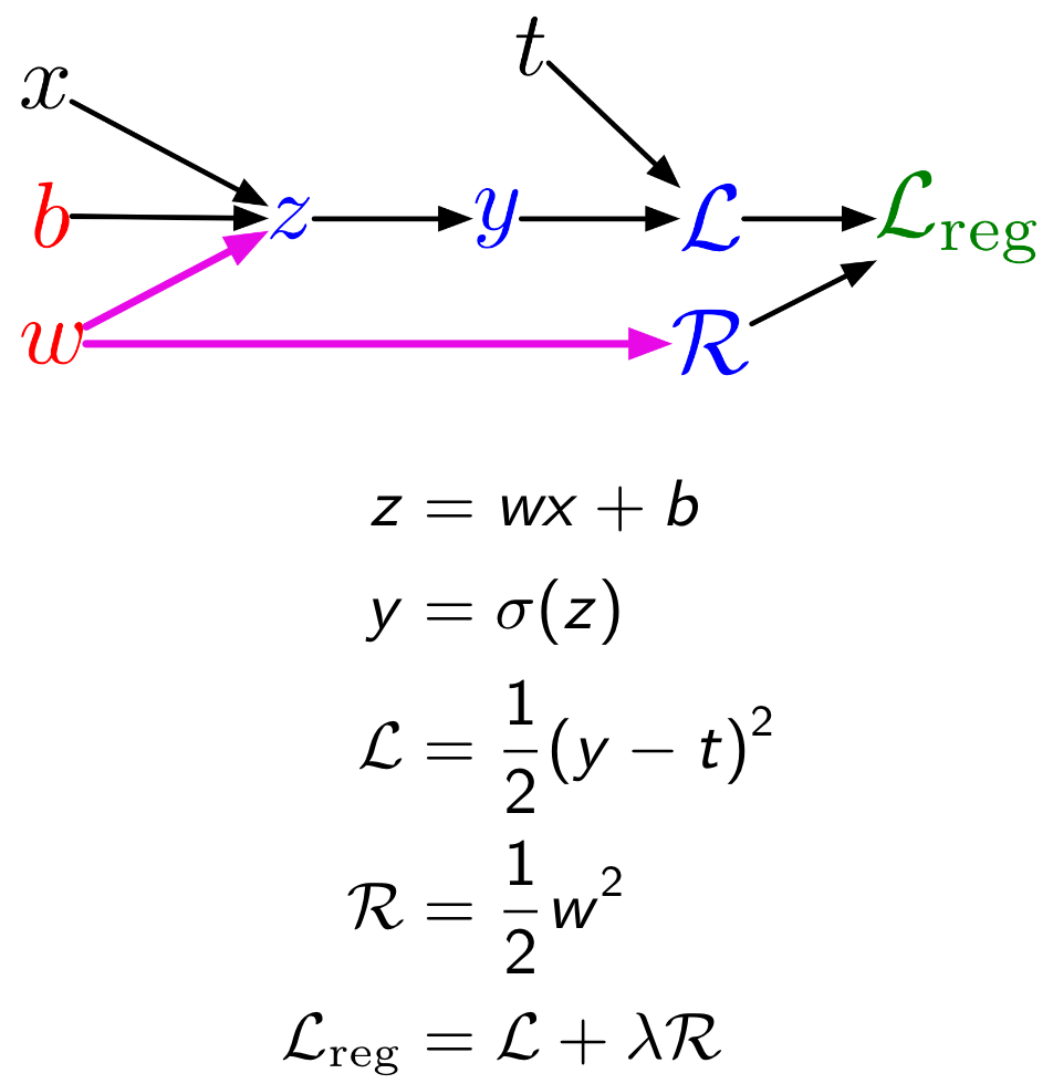
Back-propagation is an efficient way to calculate these gradients using the chain rule. We represent the application of a model to its inputs as a computation graph: nodes represent variables and edges represent functions which operate on them.

For example, a simple logistic regression model can be represented as the following graph:

Now let’s generalize this idea. Assume a graph with variables and functions which compute them from other variables.

The graph is directional, so we can define a topological order of the graph (parents before children): , where is the final objective value.

We’ll also introduce the notation , which is simply a shorthand for the gradient of the loss with respect to a particular variable. We’ll assume a scalar loss, so this expression has the same dimensions as the variable .

Forward pass

In the forward pass, we evaluate the function represented by the entire computation graph. Given the formalism from the previous section, we can write the algorithm for a forward pass as follows:

1. For :
2. Get graph parents of current node:
3. Evaluate function at current node:

Backward pass

In the backward pass, our goal is to compute the gradient of the loss with respect to each one of the variables (nodes) defined in the computation graph.

We do this by simply traversing the graph in reverse and applying the chain rule:

1. Set .
2. For :
3. Get the graph children of current node:
4. Apply the chain rule:

Notice the sum over a node’s children in the last expression. When a computation node’s output is used by more than one other node (i.e., it has more than one child in the graph), we must sum the incoming gradients from these children. This again arises directly from the chain rule.

The expression is known as a “vector”-Jacobian product (VJP). Notice that is a vector (because the loss is scalar), and is the Jacobian matrix of the two variables and , so the resulting VJP is also a vector.

Modularity

Backpropagation easily lends itself to a modular and efficient implementation.

Backpropagation is modular in the sense that nodes in the computation graph only need to know how to calculate the derivatives of the functions on their incoming edges. These derivatives are then passed to the parent nodes, which can then also only need to know how to calculate their own derivatives.

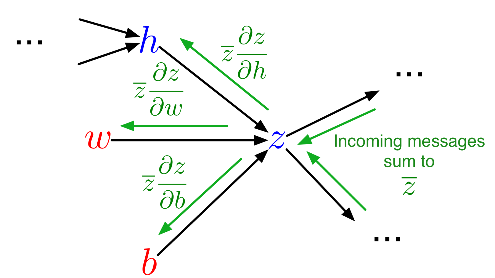
(note: in the figure, means in our notation)

This modularity means that a computation graph can be composed of loosely coupled nodes, each just having to know how to compute its own forward pass (evaluate its function) and backward pass (compute the derivative of whatever function it implements).

Efficiency

Backpropagation is also an efficient algorithm, in the sense that we only have to compute each once. Moreover, there’s never a need to construct a full Jacobian for a node, and we can instead calculate the VJP directly since that’s what’s actually needed.

Modern automatic-differentiation packages such as PyTorch’s autograd utilize exactly these tricks to implement backpropagation in a powerful and flexible way.

Conclusion

We’ve covered the two basic things you need to train a model:

• Computing the gradient of the loss w.r.t. to each parameter.
• Using said gradient to update said parameter.

Hopefully, this post gave you a basic overview of the fundamentals, and will make it easier to dive deeper when necessary.